HNSW vs IVFFlat: Choosing and Tuning Your pgvector Index
The two pgvector index types, the exact params that trade recall for speed, and how to tune them.
AI-drafted, reviewed by Muhammad Qasim Hammad on July 21, 2026. See our AI disclosure.
Table of contents
You added the vector column, you loaded your embeddings, and your similarity query works. Then the table grows and the same query crawls. In pgvector the fix is an index, and you have exactly two real choices whose trade-offs almost every tutorial skips.
HNSW vs IVFFlat: which pgvector index should you pick?#
The choice between HNSW and IVFFlat comes down to build cost versus query performance. HNSW is a graph index with the best speed-recall tradeoff, but it builds slower and uses more memory. IVFFlat clusters your vectors, builds faster, and uses less memory, yet you must create it after the data is loaded.
Both are approximate, so both give up a little recall for speed compared to an exact scan. The pgvector README is blunt about the headline difference: HNSW "has better query performance than IVFFlat (in terms of speed-recall tradeoff), but has slower build times and uses more memory." That one sentence decides most cases, but the tuning underneath it is where posts go quiet.
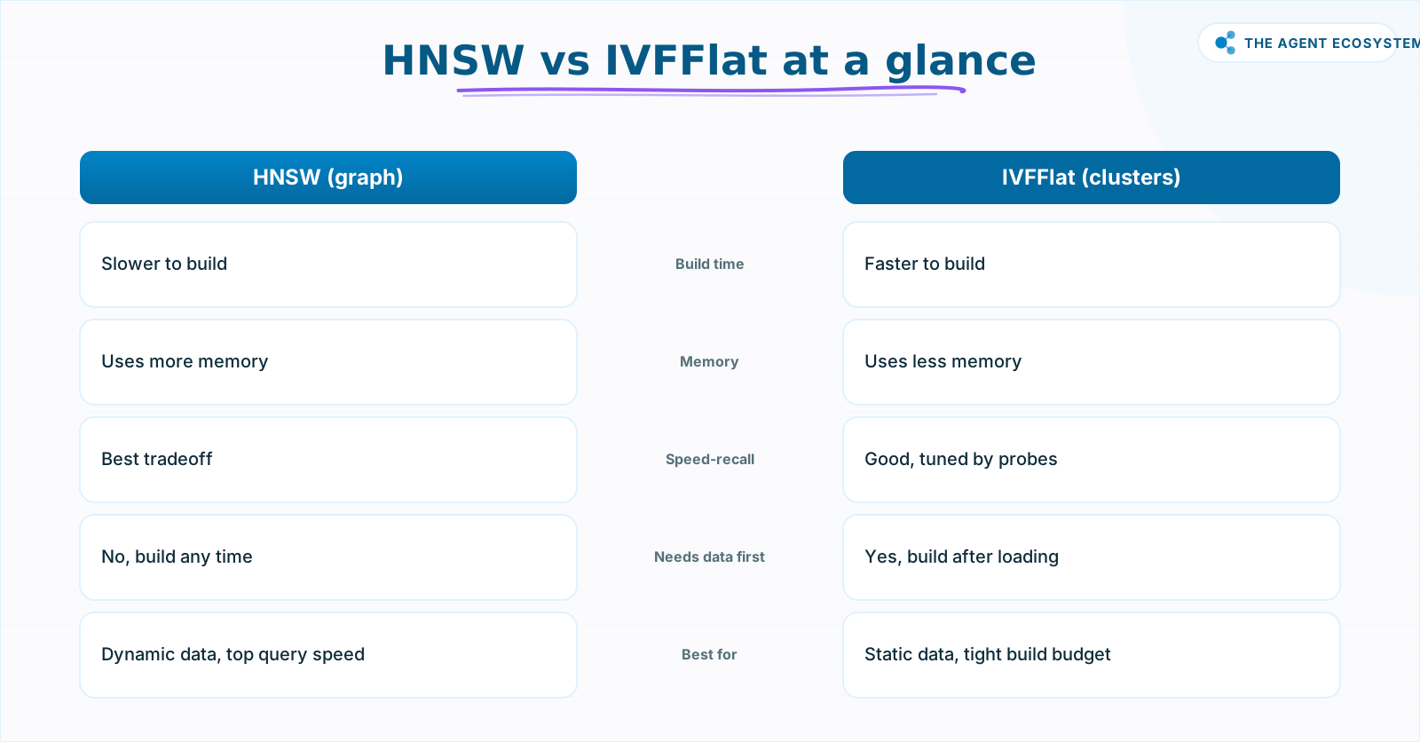 HNSW wins the speed-recall tradeoff; IVFFlat builds faster and uses less memory. Choose by your data shape and build budget.
Keep the shape of each index in mind. HNSW links every vector to a handful of neighbors across layers, so a search walks the graph toward the closest matches. IVFFlat splits the space into clusters and only scans the few nearest ones. The knobs you tune, and the failure modes, follow directly from those two structures.
How does HNSW work, and what tunes it?#
HNSW builds a layered graph where each node connects to its nearest neighbors, and a query hops through that graph toward the closest vectors. Two build parameters shape the graph, and one query parameter trades recall for speed at search time. You do not need to know your row count up front to build it.
At build time, m sets the max connections per layer and defaults to 16, while ef_construction sets the candidate-list size while building and defaults to 64. A larger m or ef_construction builds a richer graph with better recall, at the cost of build time and memory. At query time, hnsw.ef_search defaults to 40 and controls how wide the search looks; you raise it per session with SET hnsw.ef_search = 100 when you want more recall.
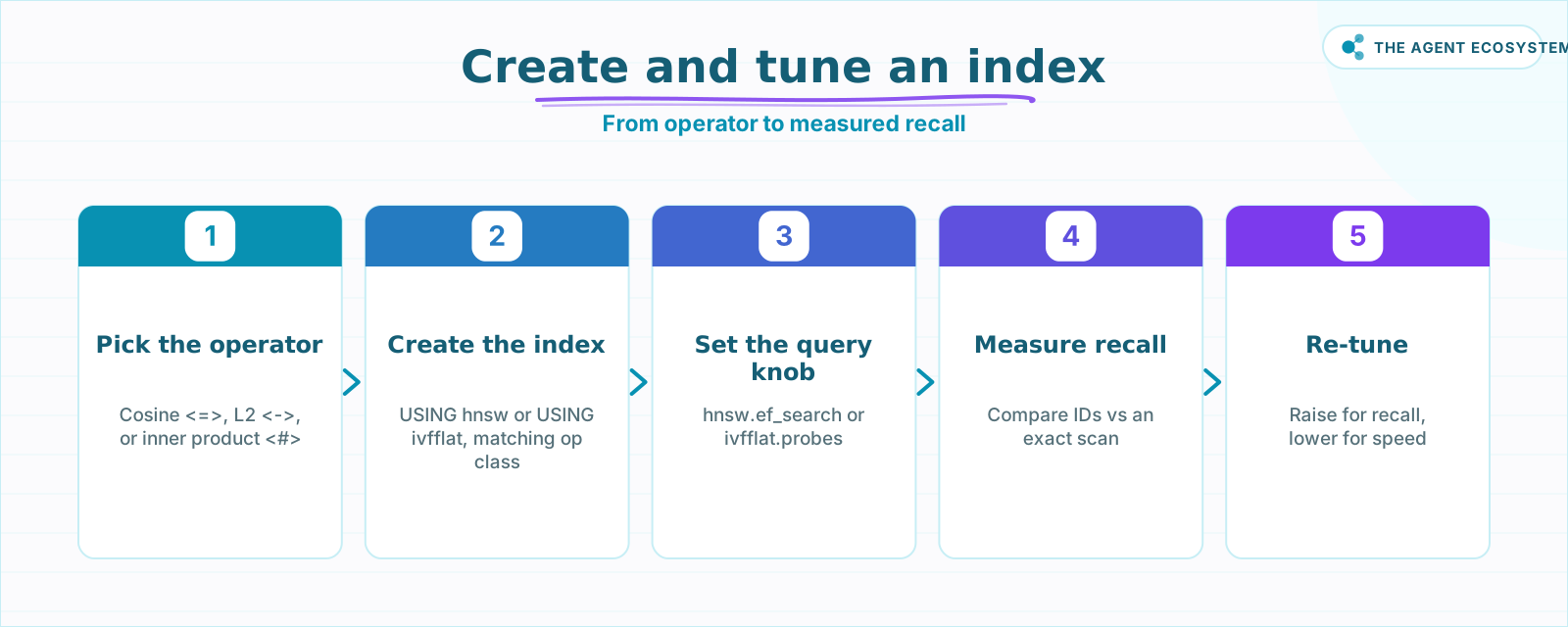 The loop is the same for both index types: create, set the query knob, measure recall against exact search, then re-tune.
That last knob is the one you reach for most. Because ef_search is a session setting, you can dial recall up for a critical query path and leave it low elsewhere, without rebuilding anything. The build parameters are fixed at index creation, so getting m roughly right the first time saves you a rebuild later.
How does IVFFlat work, and why build it after loading?#
IVFFlat partitions your vectors into lists clusters during the build, then at query time it probes only the nearest few clusters instead of every row. Because the clusters are learned from the data itself, an IVFFlat index built on an empty or tiny table learns bad clusters, so you must create it after the table already holds representative rows.
The pgvector README gives a starting point for lists: use rows / 1000 for up to 1M rows, and sqrt(rows) above that. At query time, ivfflat.probes defaults to 1, and raising it scans more clusters for better recall at the cost of speed. So IVFFlat has one build knob (lists) and one query knob (probes), which makes it simpler to reason about than HNSW, if you can pay the rebuild-on-empty tax.
The catch is real churn. If your data changes constantly, the clusters drift and recall slips until you rebuild. That is exactly why the same README steers dynamic workloads toward HNSW, whose graph tolerates inserts far better without a full rebuild.
Which distance operator, and does it have to match?#
Both indexes support the same three distance operators, and the operator you query with must match the operator class you built the index for. Cosine distance uses <=>, L2 (Euclidean) uses <->, and inner product uses <#>. Build a cosine index but query with L2 and the planner silently skips the index.
That silent skip is a classic pgvector footgun. Your query still returns rows, so nothing looks broken, but you have quietly fallen back to a slow exact scan on every row. Pick the operator that matches how your embedding model measures similarity, then build the matching operator class (vector_cosine_ops, vector_l2_ops, or vector_ip_ops) so the index actually gets used.
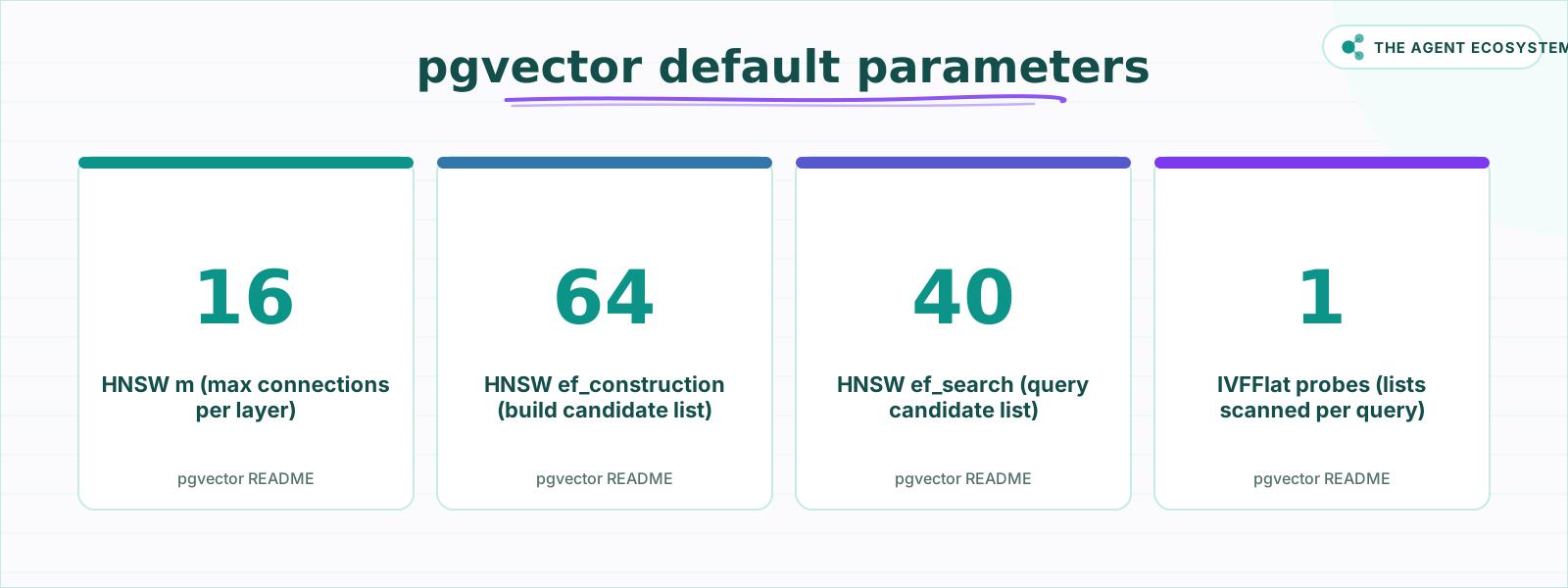 The defaults from the pgvector README. Raise the query-time knobs (ef_search, probes) to lift recall at the cost of speed.
Here is the same information as a cheat-sheet you can keep next to your migration file:
| Concern | HNSW | IVFFlat |
|---|---|---|
| Structure | Layered neighbor graph | Clustered lists |
| Build params | m (16), ef_construction (64) | lists (rows/1000 up to 1M) |
| Query param | hnsw.ef_search (40) | ivfflat.probes (1) |
| Build before data? | Yes | No, load data first |
| Best for | Dynamic data, top speed | Static data, lean memory |
How do you tune and verify your chosen index?#
Tune by moving one query-time knob and measuring recall against exact search. Raise hnsw.ef_search or ivfflat.probes for more recall, lower it for more speed. To measure recall, run the query with the index and against an exact scan, then compare how many of the same IDs come back.
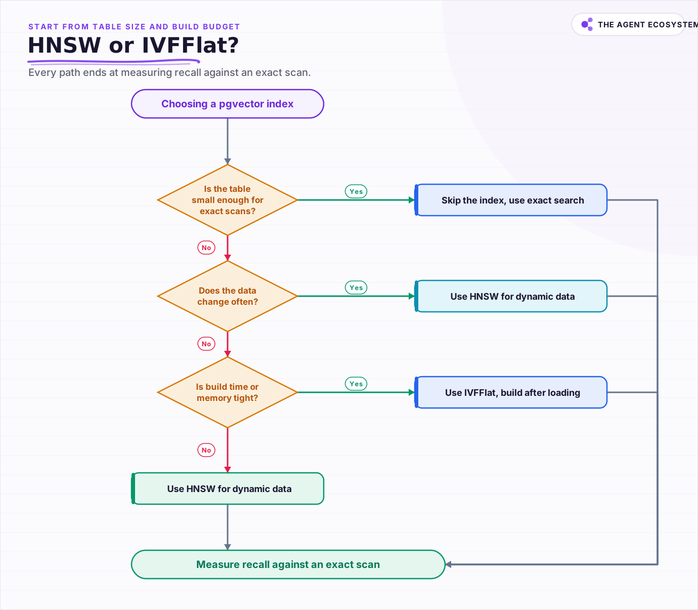 Start from table size and build budget; every path ends at measure recall against an exact scan before you trust it.
Recall is not a vibe; it is the overlap between your approximate results and the true nearest neighbors from an exact scan. If your index returns 8 of the true top 10, that is 0.8 recall, or 80%. Decide the recall you actually need for the task, tune until you hit it, and only then chase latency. If you are still choosing a vector store at all, our comparison of pgvector against Chroma and Qdrant covers when Postgres is the right home for these indexes in the first place.
So which index wins for your workload?#
Neither index wins outright; the right pick is the one that matches your data and build budget. Choose HNSW for the best query performance and for data that changes often, since its graph tolerates inserts. Choose IVFFlat when build time and memory are tight and the data is mostly static, and remember to build it after loading.
Whichever you pick, treat the defaults as a starting line, not a finish. Build the index, set one query-time knob, measure recall against an exact scan, and re-tune until both recall and latency sit where the task needs them. Verify the current parameter names against the pgvector README before you standardize a migration, because this project moves fast.
Frequently asked questions
What is the difference between HNSW and IVFFlat in pgvector?
Do I need an index at all in pgvector?
What are the default HNSW parameters in pgvector?
How do I set the lists parameter for IVFFlat?
Does the distance operator have to match the index?
Sources
Primary references and vendor documentation used while drafting and reviewing this article.
Written by

Muhammad Qasim Hammad is an AI agent and automation expert and the founder of Cart Gaze LLC (cartgaze.com). He builds product for the love of it: when an idea lands, a working prototype is usually running within hours, built with the same AI agents and automations he sells. He puts his own output at roughly 20× what it was before agents, and the Agentic OS behind this site is the working proof, documented in public with the tools he actually ran and what they really cost.
AI & Automation Services
Want a pipeline like this running in your business?
I'm Qasim — I design and ship AI agents and n8n automations for solo operators and small teams. Tell me what's eating your team's week, and I'll scope a fix.
Related reading
n8n Pinecone vs Supabase Vector Store: Which to Pick
The n8n Pinecone Vector Store and Supabase Vector Store nodes wire into an agent the same way, but one is a managed service and one is Postgres you run. Here is how their free tiers, cost at scale, latency, and node wiring compare, and when to pick each for RAG.

Embedding Dimensions and Cost: Bigger Vectors, Better RAG?
You assumed more embedding dimensions mean better retrieval, and you are about to over-pay on vector storage for a margin you will never notice. OpenAI's own numbers show text-embedding-3-large at 256 dims beating ada-002 at 1536. Here is what dimensions cost and how to pick a
pgvector vs Chroma vs Qdrant: Choosing a Vector Database for RAG
Compare pgvector, Chroma, and Qdrant for local RAG pipelines. Get the three-line decision: already on Postgres, use pgvector; prototyping locally, use Chroma; need scale or heavy filtering, use Qdrant.
Build a Vector Store in n8n (Embeddings for RAG)
Build an n8n vector store that retrieves your own documents by meaning, not keywords. Embedding 1,000 docs costs ~1.3 cents; Supabase free-tier storage costs $0. Full node wiring and step-by-step setup inside.
Hybrid Search for RAG in n8n: BM25 + Vector, and When to Use Each
Vector search nails meaning but misses exact tokens like SKUs, error codes, and function names. Hybrid search adds a BM25 keyword leg and fuses both with Reciprocal Rank Fusion. Here is when each wins and how to wire it in n8n with Qdrant or pgvector.
Keeping RAG Indexes Fresh: Incremental Updates Without Full Re-Embeds
A RAG bot is only as current as its last ingest, and re-embedding the whole corpus nightly pays for thousands of unchanged documents to pick up a handful of edits. This is the incremental alternative: hash to detect changes, upsert by stable chunk IDs, tombstone deletes, and